Plot an ABN graphic

Plot an ABN DAG using formula statement or a matrix in using Rgraphviz through the graphAM class.

Usage

plotAbn(dag, data.dists=NULL, markov.blanket.node=NULL, fitted.values=NULL,
               digits=2, edge.strength=NULL, edge.strength.lwd=5, edge.direction="pc",
               edge.color="black", edge.linetype="solid", edge.arrowsize=0.6,
               edge.fontsize=node.fontsize, node.fontsize=12,
               node.fillcolor=c("lightblue", "brown3", "chartreuse3"),
               node.fillcolor.list=NULL,
               node.shape=c("circle", "box", "ellipse", "diamond"),
               plot=TRUE , ...)

Arguments

dag: a matrix or a formula statement (see details for format) defining the network structure, a Directed Acyclic Graph (DAG). Note that rownames must be set or given in data.dists.
data.dists: a named list giving the distribution for each node in the network, see details.
markov.blanket.node: name of variables to display its Markov blanket.
fitted.values: modes or coefficents outputted from fitAbn.
digits: number of digits to display the fitted.values.
edge.strength: a named matrix containing evaluations of edge strength which will change the arcs width (could be Mutual information, p-values, number of bootstrap retrieve samples or the outcome of the linkStrength).
edge.strength.lwd: maximum line width for edge.strength.
edge.direction: character giving the direction in which arcs should be plotted, pc (parent to child) or cp (child to parent) or undirected.
edge.color: the colour of the edge.
edge.linetype: the linetype of the edge. Defaults to "solid". Valid values are the same as for the R's base graphic parameter lty.
edge.arrowsize: the thickness of the arrows. Not relevant if arc.strength is provided.
edge.fontsize: the font size of the arcs fitted values.
node.fontsize: the font size of the nodes names.
node.fillcolor: the colour of the node. Second and third element is used for the Markov blanket and node of the Markov blanket.
node.fillcolor.list: the list of node that should be coloured.
node.shape: the shape of the nodes according the Gaussian, binomial, Poisson and multinomial distributions.
plot: logical variable, if set to TRUE then the graph is plotted.
...: arguments passed to the plotting function.

Value

A rendered graph, if plot=TRUE. The graphAM object is returned invisibly.

Details

By default binomial nodes are squares, multinomial nodes are empty, Gaussian nodes are circles and poison nodes are ellipses.

The dag can be provided using a formula statement (similar to glm). A typical formula is ~ node1|parent1:parent2 + node2:node3|parent3.

The construction is based on the graph package. Properties of the graph can be changed after the construction, see ‘Examples’.

Examples

# Define distribution list
dist <- list(a = "gaussian",
             b = "gaussian",
             c = "gaussian",
             d = "gaussian",
             e = "binomial",
             f = "binomial")

# Define a matrix formulation
edge_strength <- matrix(c(0, 0.5, 0.5, 0.7, 0.1, 0,
                          0, 0, 0.3, 0.1, 0, 0.8,
                          0, 0, 0, 0.35, 0.66, 0,
                          0, 0, 0, 0, 0.9, 0,
                          0, 0, 0, 0, 0, 0.8,
                          0, 0, 0, 0, 0, 0),
                        nrow = 6L,
                        ncol = 6L,
                        byrow = TRUE)

## Naming of the matrix
colnames(edge_strength) <- rownames(edge_strength) <- names(dist)

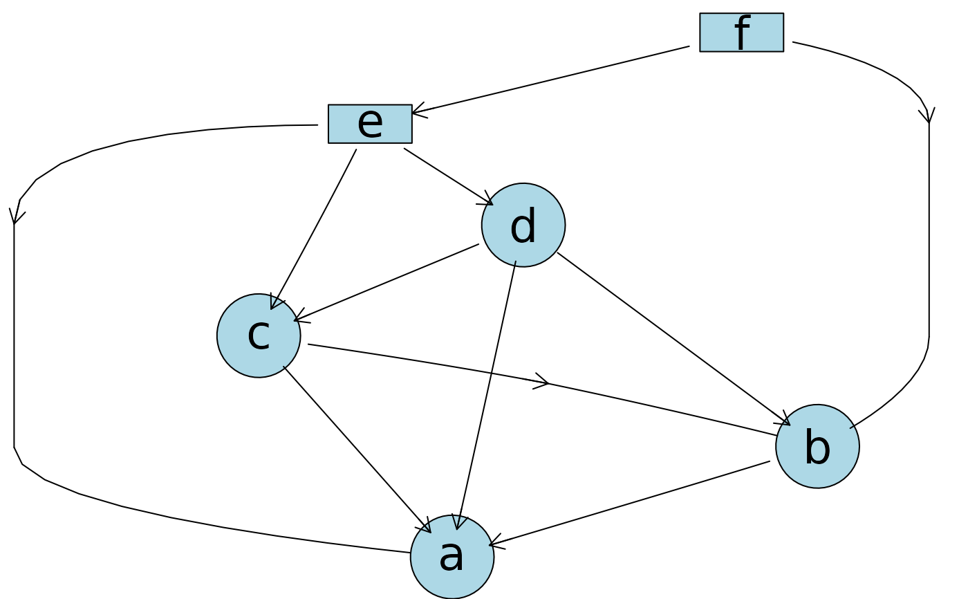
## Plot form a matrix
plotAbn(dag = edge_strength,
        data.dists = dist)


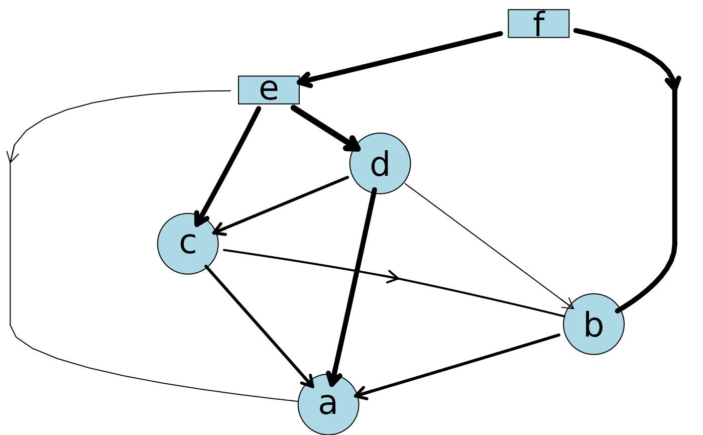
## Edge strength
plotAbn(dag = ~ a | b:c:d:e + b | c:d:f + c | d:e + d | e + e | f,
        data.dists = dist,
        edge.strength = edge_strength)


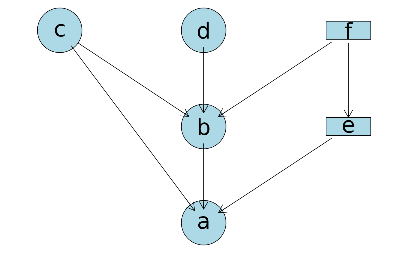
## Plot from a formula for a different DAG!
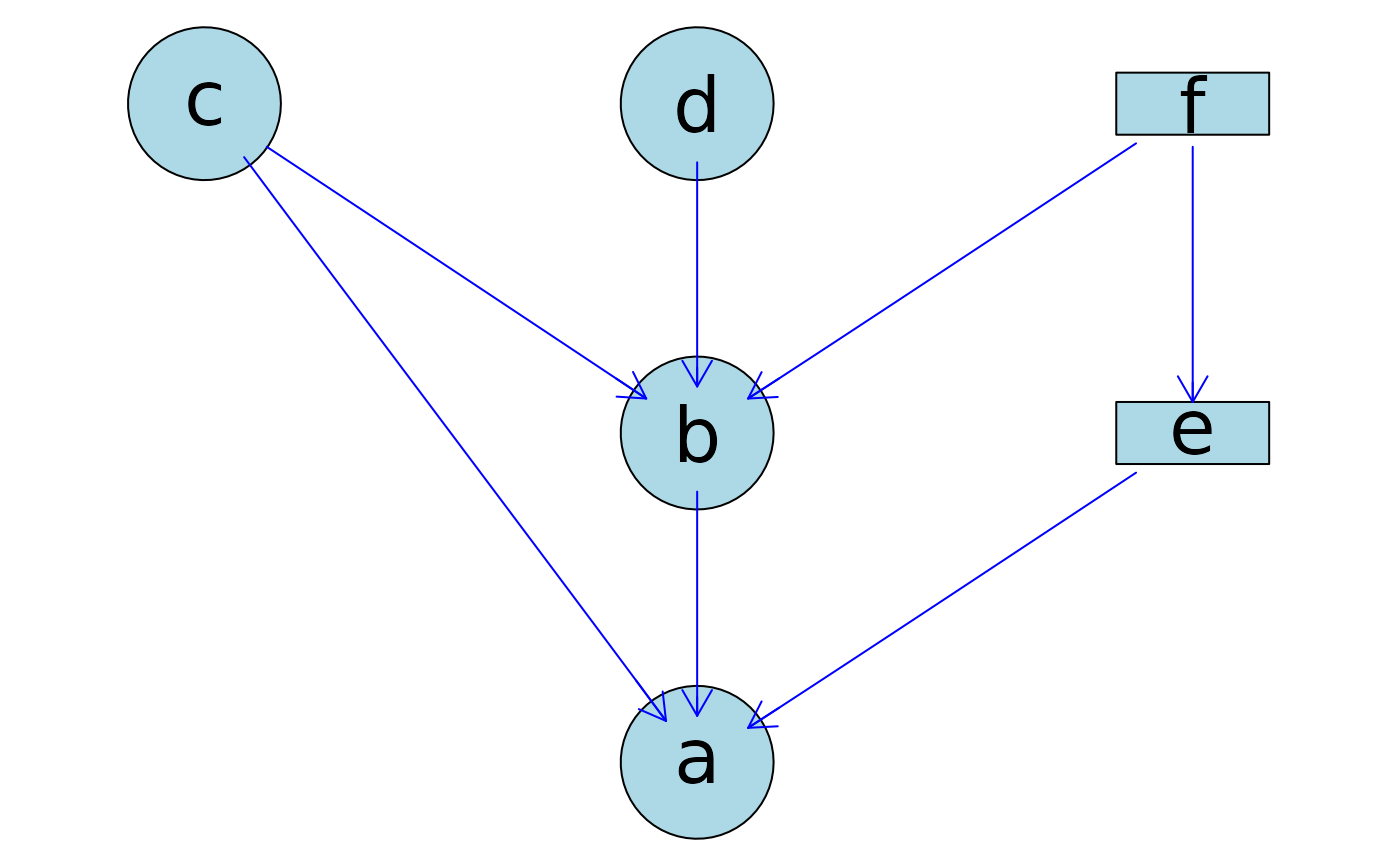
plotAbn(dag = ~ a | b:c:e + b | c:d:f + e | f,
        data.dists = dist)


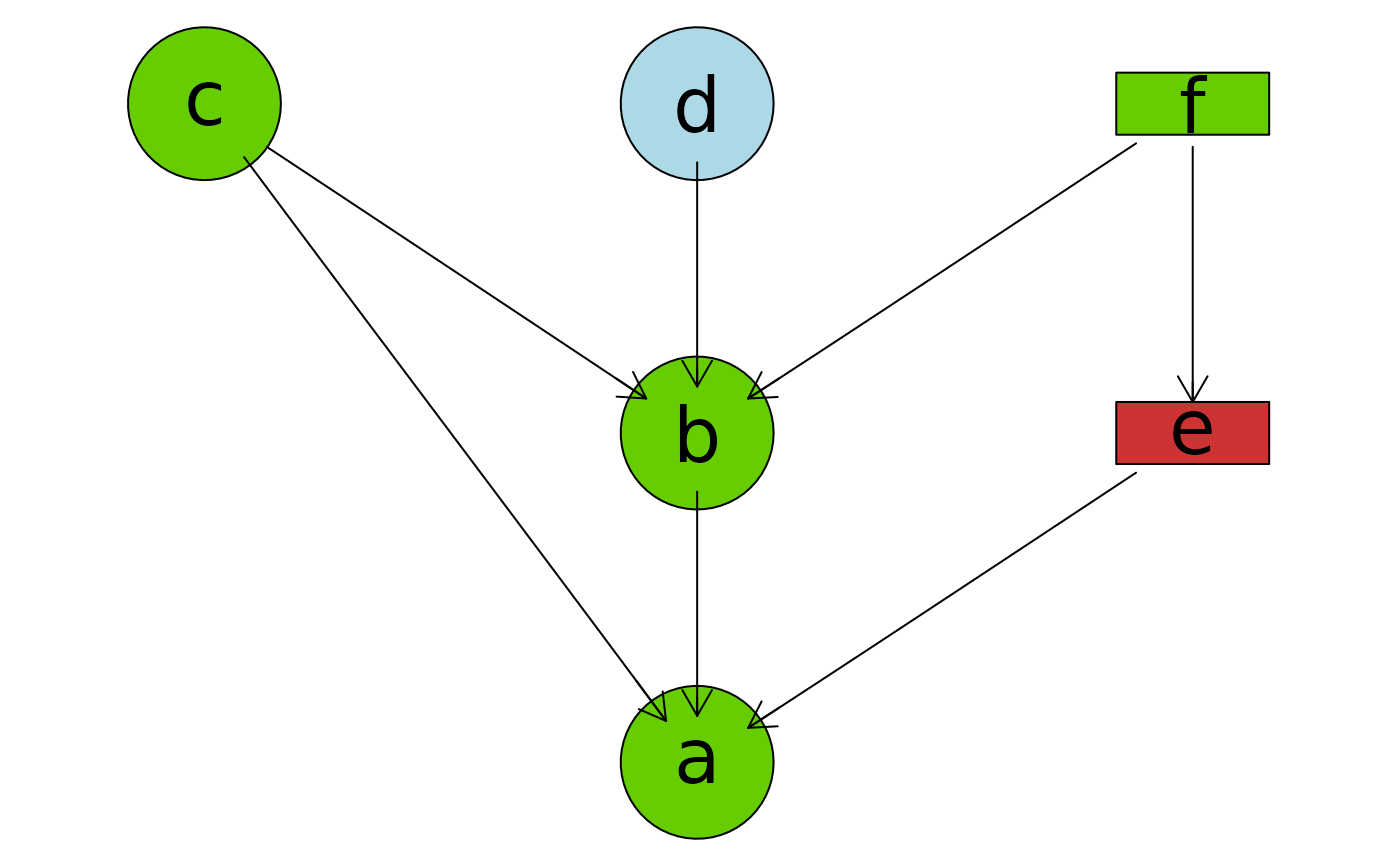
## Markov blanket
plotAbn(dag = ~ a | b:c:e + b | c:d:f + e | f,
        data.dists = dist,
        markov.blanket.node = "e")


## Change col for all edges
tmp <- plotAbn(dag = ~ a | b:c:e + b | c:d:f + e | f,
               data.dists = dist,
               plot = FALSE)
graph::edgeRenderInfo(tmp) <- list(col = "blue")
Rgraphviz::renderGraph(tmp)


## Change lty for individual ones. Named vector is necessary
tmp <- plotAbn(dag = ~ a | b:c:e + b | c:d:f + e | f,
               data.dists = dist,
               plot = FALSE)
edgelty <- rep(c("solid", "dotted"), c(6, 1))
names(edgelty) <- names(graph::edgeRenderInfo(tmp, "col"))
graph::edgeRenderInfo(tmp) <- list(lty = edgelty)
Rgraphviz::renderGraph(tmp)

Usage

Arguments

Value

Details

See also

Examples